(DMAT) Received June 20, 2023.
The natural world is full of large systems of interacting units. A human brain, for example, contains around 86 billion (86 · 10^{9}) neurons whose activities evolve in time as a function of the activities of the neurons they are connected to. An ecosystem can also be regarded as an interacting network in which the units are the different species and their abundances are variables that depend on the abundances of the species they interact with. A social network is another environment through which information, opinion or diseases can spread or disappear depending on the structure of its interactions.
Systems as the ones defined by these examples are usually dubbed “complex”, a broad term that is used to emphasize the fact that their behavior is often difficult to study and predict. A natural question to ask is whether a generic complex system composed of N interacting units or nodes (e.g., neurons, species, individuals) can be reduced to a simpler system composed of n ≪ N units. In other words: if one can construct a smaller system that is easier to treat and understand while preserving some of the characteristic properties of the original system. Imagine an ecosystem in which the species’ abundances are relatively stable in time. These abundances may change smoothly as some perturbation is introduced, for example a change in the average annual temperature, which alters the capacity of some species to survive or reproduce. If the perturbation is too strong, however, this equilibrium could disappear and the system might abruptly drift to a state characterized by a partial or total species extinction. It is thus important to know what is the critical temperature at which such a catastrophe occurs, and we would like a reduced version of the system to have an analogous transition at roughly the same temperature. Being able to construct such a reduced system is not only useful for practical reasons (i.e., simulating it and predicting its behavior using less resources) but also from a purely theoretical point of view, because in doing so we can learn about the inner workings of the original system and the reduced dimension n is a measure of the “effective complexity” that characterizes it.
In 2016, Gao, Barzel and Barabási [1] proposed a way to reduce a system on N nodes whose activity evolves in time according to
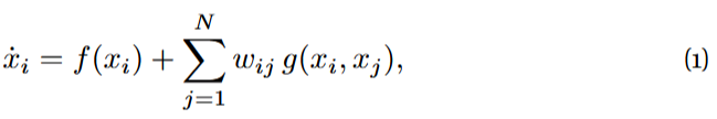
where x_{i} = x_{i}(t) is the activity of node i at time t and w_{ij} > 0 stands for the weight of the positive interaction from node j to node i. Functions f and g define the nodes’ self-dynamics and the dynamical coupling between pairs of nodes, respectively.
They proposed to reduce the system to a system of dimension n = 1 whose only effective (or macroscopic) activity Xeff
is a linear combination of the activities in the original system according to
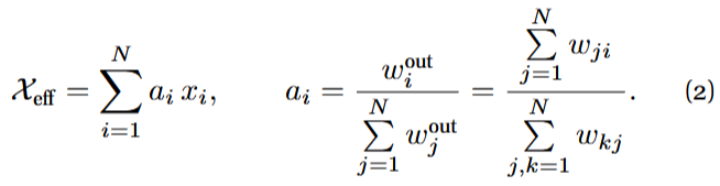
The quantity ![]() is the (weighted) out-degree of node i. Eq. (2) thus states that the effective activity is a weighted average of the microscopic activities according to a positive vector
is the (weighted) out-degree of node i. Eq. (2) thus states that the effective activity is a weighted average of the microscopic activities according to a positive vector ![]() with sum 1 whose entries are proportional to the nodes’ out-degrees. The authors showed that X_{eff} approximately follows an ODE which has the same structure as the original dynamics:
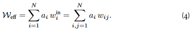
with sum 1 whose entries are proportional to the nodes’ out-degrees. The authors showed that X_{eff} approximately follows an ODE which has the same structure as the original dynamics:
![]()
the effective interaction weight W_{eff} being the weighted average, according to the same vector a, of the in-degrees:
They argued that such a one-dimensional reduction can capture the tipping points of several complex systems as different parameters are perturbed.
Despite some systems may be effectively reduced this way, it is likely that other systems will not be properly represented by a system of dimension just one. So can we generalize this result in some way? Can we construct a set of n ≪ N linear effective variables —called observables from now on— and a reduced matrix of interactions ![]() whose dynamics, at least approximately, has the same form as the original one? In what follows I will outline a possible way to that end (exposed in detail in Ref. [2]), assuming that the original system’s evolution is given by Eq. (1). Fig. 1 provides a visual sketch of the process.
whose dynamics, at least approximately, has the same form as the original one? In what follows I will outline a possible way to that end (exposed in detail in Ref. [2]), assuming that the original system’s evolution is given by Eq. (1). Fig. 1 provides a visual sketch of the process.
Imagine that we start by partitioning the units in our network according to their connectivity properties so that nodes within a group connect similarly to nodes in other groups. A neuronal network, for instance, might contain functional modules composed of neurons that are densely connected among them but sparsely connected to neurons in other modules. In an ecological network, species that exploit similar niches (and thus interact with other species in a similar way) could be grouped together. If we do not have any information about the presence of modules in the network, we could use a community-detection algorithm on the matrix of interactions![]() and try to identify them.
and try to identify them.
Our reduced system will have as many variables as the number of groups in the partition, n. We denote by G_{1}, · · · , G_{n} these groups. We require the ν-th observable to be a weighted average of the activities within group G_{ν} , that is, denoting by![]() the size of G_{ν} , we want to find a non-negative vector
the size of G_{ν} , we want to find a non-negative vector ![]() with sum 1 and construct from it the observable associated to G_{ν},
with sum 1 and construct from it the observable associated to G_{ν},
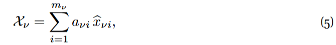
where ![]() is the vector of activities of nodes in group G_{ν}. We call the vectors a_{1}, · · ·, a_{n} the reduction vectors.
is the vector of activities of nodes in group G_{ν}. We call the vectors a_{1}, · · ·, a_{n} the reduction vectors.
The next step is to write down the exact ODE for the evolution of the ν-th observable, which is a function of ![]() and
and ![]() for i ∈ {1, · · · , m_{ν}}, ρ ∈ {1, · · · , n} and j ∈ {1, · · · , m_{ρ}}, and, generically, cannot be expressed as a function of the observables only. To approximately close the observables’ dynamics, we hypothesize that, if the node partition is defined properly, nodes within the same group will have similar activities. Thus, these activities will be close to the corresponding observable and it makes sense to use first-order Taylor approximations of
for i ∈ {1, · · · , m_{ν}}, ρ ∈ {1, · · · , n} and j ∈ {1, · · · , m_{ρ}}, and, generically, cannot be expressed as a function of the observables only. To approximately close the observables’ dynamics, we hypothesize that, if the node partition is defined properly, nodes within the same group will have similar activities. Thus, these activities will be close to the corresponding observable and it makes sense to use first-order Taylor approximations of ![]() and
and ![]() around X_{ν} and (X_{ν} , X_{ρ}), respectively. In doing so, we obtain an approximate system of ODEs that will not be closed unless the reduction vectors fulfill the following conditions:
around X_{ν} and (X_{ν} , X_{ρ}), respectively. In doing so, we obtain an approximate system of ODEs that will not be closed unless the reduction vectors fulfill the following conditions:
![]()
where ![]() is the m_{ν} × m_{ν} diagonal matrix whose diagonal is the vector of in-degrees of nodes in G_{ν} taking into account connections coming from G_{ρ} only, and W_{νρ} is the m_{ν} × m_{ρ} matrix of interactions from nodes in G_{ρ} to nodes in G_{ν} . The scalars μ_{νρ} and λ_{νρ} are additional parameters to be found. Eqs. (6a),(6b) are called the compatibility equations. They impose constraints on the reduction vectors.
is the m_{ν} × m_{ν} diagonal matrix whose diagonal is the vector of in-degrees of nodes in G_{ν} taking into account connections coming from G_{ρ} only, and W_{νρ} is the m_{ν} × m_{ρ} matrix of interactions from nodes in G_{ρ} to nodes in G_{ν} . The scalars μ_{νρ} and λ_{νρ} are additional parameters to be found. Eqs. (6a),(6b) are called the compatibility equations. They impose constraints on the reduction vectors.
Once the compatibility equations are fulfilled, the approximate reduced dynamics has the form
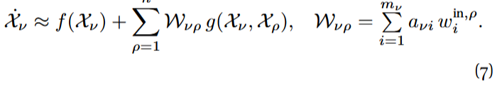
The matrix ![]() is thus the effective interaction matrix in the reduced system. Notice that both the approximate reduced dynamics and W have the same form as Eqs. (3) and (4) proposed by Gao et al., for an arbitrary n. The difference with their approach is the construction of the observable vectors, as we will show now.
is thus the effective interaction matrix in the reduced system. Notice that both the approximate reduced dynamics and W have the same form as Eqs. (3) and (4) proposed by Gao et al., for an arbitrary n. The difference with their approach is the construction of the observable vectors, as we will show now.
In our approach, we must solve the compatibility equations to find the reduction vectors. If the nodes in G_{ν} have similar connectivity properties, their in-degrees from G_{ρ} will be close to one another and K_{νρ} will be close to a multiple of the identity matrix so Eq. (6a) can be assumed to be automatically fulfilled. We thus concentrate in solving Eq. (6b) for all ν, ρ, that is,
![]()
For n = 1, this is a single equation and it states that the vector ![]() must be an eigenvector of the transposed connectivity matrix W^{T} . If this matrix is positive, since we ask the reduction vector to be non-negative, then it has to be the dominant, or Perron-Frobenius, eigenvector of W^{T}, normalized to have sum 1. Despite in some particular situations the normalized dominant eigenvector and the vector of normalized out-degrees proposed by Gao et al. coincide, in general they are not the same.
must be an eigenvector of the transposed connectivity matrix W^{T} . If this matrix is positive, since we ask the reduction vector to be non-negative, then it has to be the dominant, or Perron-Frobenius, eigenvector of W^{T}, normalized to have sum 1. Despite in some particular situations the normalized dominant eigenvector and the vector of normalized out-degrees proposed by Gao et al. coincide, in general they are not the same.
For n > 1, Eqs. (8) are coupled, but we can decouple them using, again, the Perron-Frobenius theorem when W is a posi tive matrix. In this case, Eqs. (8) are equivalent to the following decoupled equations:
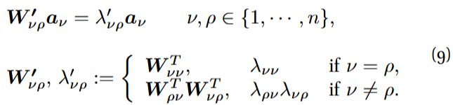
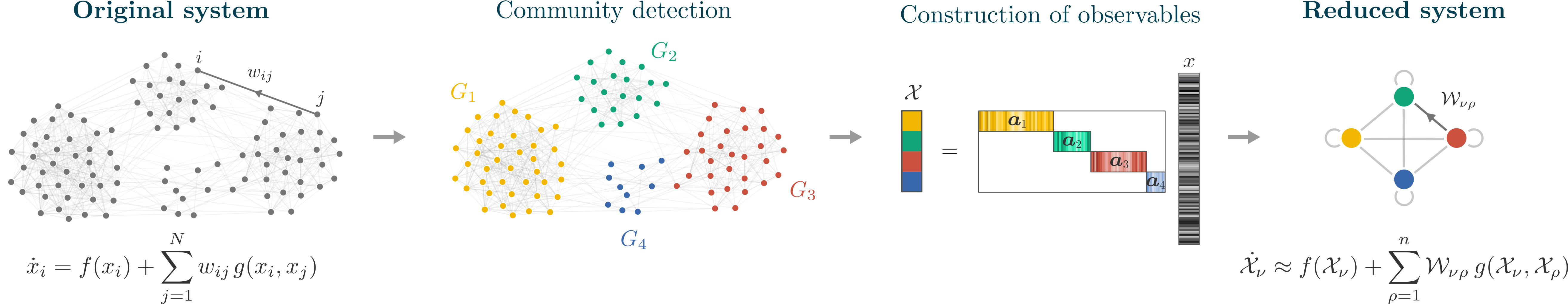
Figure 1: Schematics of the dimension-reduction strategy.
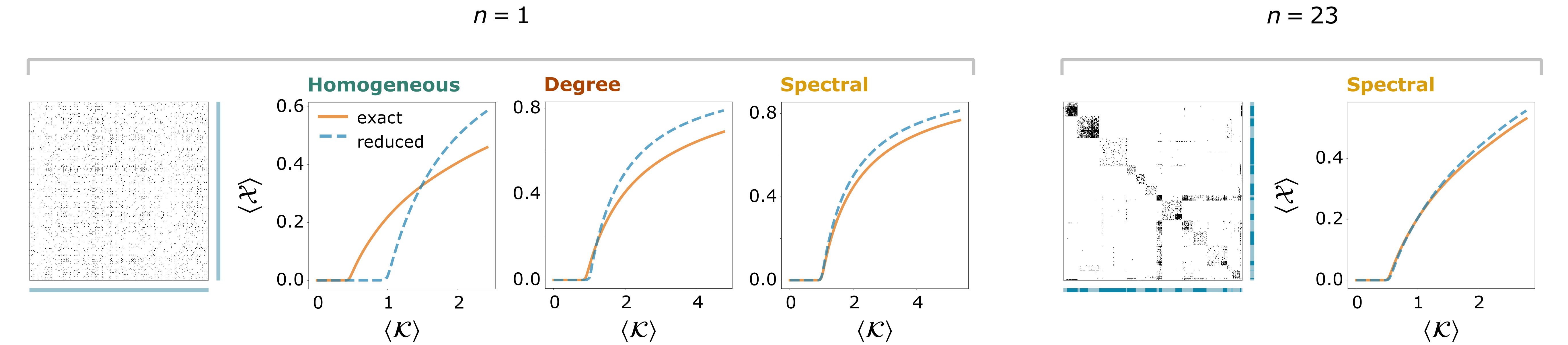
Figure 2: Dimension reduction results for a susceptible-infected-susceptible (SIS) infectious dynamics given by Eq. (1) with f (x) = −x and g(x, y) = (1 − x)y on a network based on Facebook contacts with N = 362 nodes [2]. We plot the average observable at equilibrium, ⟨X⟩, as a function of the average weighted in-degree of the reduced system, ⟨K⟩, (both of them weighted by the relative sizes of the different groups) for the exact and the reduced dynamics. The parameter ⟨K⟩ increases as a consequence of multiplying all the interaction strengths by a global factor. For n = 1 (i.e., when considering the whole network as a unique group), we compare three reductions: a homogeneous reduction in which all the nodes contribute equally to the observable (left), the degree-based reduction defined by Gao et al. [1] (middle), and our spectral reduction (right). The last diagram shows the spectral reduction results when the nodes have been partitioned into n = 23 groups.
For a fixed ν, Eqs. (9) state that ![]() has to be, simultaneously, the (normalized) dominant eigenvector of a collection of n positive matrices. Of course, such a vector will not exist in general because these matrices will not share their dominant eigenspace. To approximately solve the problem, we propose to set λ′_{νρ} to the dominant eigenvalue of W′_{νρ} (this is what it would be if there were an exact solution) and then find the vector
has to be, simultaneously, the (normalized) dominant eigenvector of a collection of n positive matrices. Of course, such a vector will not exist in general because these matrices will not share their dominant eigenspace. To approximately solve the problem, we propose to set λ′_{νρ} to the dominant eigenvalue of W′_{νρ} (this is what it would be if there were an exact solution) and then find the vector ![]() that minimizes the quadratic error associated to Eqs. (9). We call this dimension-reduction strategy the spectral reduction.
that minimizes the quadratic error associated to Eqs. (9). We call this dimension-reduction strategy the spectral reduction.
Fig. 2 shows an application of the spectral reduction to a susceptible-infected-susceptible (SIS) infectious dynamics on a friendship network obtained from Facebook contacts, where nonexisting interactions were assumed to have an arbitrary small value [2]. In this example every unit’s activity represents the probability of the node being infected. We plot the value of the average observable at equilibrium as we increase, along the x-axis, a global factor that multiplies all the interactions. There is a point from which the disease cannot be eradicated: the average observable becomes different from zero. This critical point is well predicted by the n = 1 spectral reduction, and it is better captured than when the reduction vector is either homogeneous or proportional to the vector of out-degrees. Moreover, the spectral diagram becomes more accurate as n increases.
What is the interpretation of the spectral reduction vectors for n > 1? From the decoupled compatibility equations [Eqs. (9)], we know that ![]() has to be the dominant eigenvector of a collection of matrices. The first matrix is
has to be the dominant eigenvector of a collection of matrices. The first matrix is ![]() , whose entries are the weights of the inverted interactions from nodes in G_{ν} to nodes in G_{ν} . The other matrices are
, whose entries are the weights of the inverted interactions from nodes in G_{ν} to nodes in G_{ν} . The other matrices are ![]() for every ρ ≠ ν, whose entries represent the weight sum of all the inverted 2-step paths from nodes in G_{ν} to nodes in G_{ν} going through nodes in G_{ρ}. The i-th component of the (normalized) dominant eigenvector of a non-negative matrix is the so-called “eigenvector centralitiy” of node i in the corresponding network: a measure of the relative importance of the node in the network (a variant of which is used by Google to rank webpages upon a search, for example).
for every ρ ≠ ν, whose entries represent the weight sum of all the inverted 2-step paths from nodes in G_{ν} to nodes in G_{ν} going through nodes in G_{ρ}. The i-th component of the (normalized) dominant eigenvector of a non-negative matrix is the so-called “eigenvector centralitiy” of node i in the corresponding network: a measure of the relative importance of the node in the network (a variant of which is used by Google to rank webpages upon a search, for example).
In summary, our findings suggest that in order to reduce the dynamics by means of grouping nodes and defining linear observables within the groups, the contribution of each node to its corresponding observable should be the relative eigenvector centrality of the node within that group, with this centrality taking into account both direct (1-step) and indirect (2-step) interactions via nodes in other groups.
References
[1] J. Gao, B. Barzel, and A. L. Barabási, Universal resilience patterns in complex networks, Nature 530 (2016), 307–312.
[2] M. Vegué, V. Thibeault, P. Desrosiers, and A. Allard, Dimension reduction of dynamics on modular and heterogeneous directed networks, PNAS Nexus 2 (2023), no. 5, 1-16.