(Maria de Maeztu fellow at CRM) Received September 18, 2023.
Computer Vision is the area of Artificial Inteligence that focuses on computer perception and processing of images. One of the main problems that arise in this area is the so called Structure-from-motion (SfM) problem or 3D-image reconstruction problem, where the main goal is to create a 3D model of an object appearing in multiple two-dimensional images.
The input of the problem is a data set of images and the output is a 3D model of the scene consisting of an estimation of the relative position of the cameras and a relative position of the objects in the pictures with respect to the cameras.
Solving this problem as accurately and quickly as possible is fundamental for autonomous driving, videogames, and animation, just to name a few examples.
The SfM pipeline is depicted in Figure 1 and it has four key steps:
- Data collection.
- Matching. In this step we match points or lines in one image that are identifiable as the same point or line in another. These pairings are called correspondences.
- Camera pose. In this step, some point and line correspondences are used to estimate the relative position of the cameras.
- Triangulation. The camera positions are used to estimate the position of the world and line points whose images are the point and line correspondences obtained in the matching step.
The final 3D model is given by the camera positions and the world points and lines obtained from steps 3 and 4.
Although the input of the SfM pipeline is a set of images, at the end of Step 2 the images are forgotten and we are left with purely geometric information: correspondences of points or lines that are believed to come from the same world feature. To analyse this geometric information, the use of Algebraic Geometry is a natural choice.
Algebraic models for computer vision
In this note we will focus on algebraic varieties appearing in the Triangulation step. To understand them we start by modeling the process of taking a picture.
A camera is a function ![]() . Depending on the camera that we want to model, the definition of this function is going to change. A pinhole camera C is a linear projection from
. Depending on the camera that we want to model, the definition of this function is going to change. A pinhole camera C is a linear projection from ![]() to
to ![]() defined by a 3 × 4 matrix of full rank. For this model we assume that it is possible to take pictures of every point in space except for c = ker(C), which is called the camera center and, intuitively, represents the position of the camera in the world.
defined by a 3 × 4 matrix of full rank. For this model we assume that it is possible to take pictures of every point in space except for c = ker(C), which is called the camera center and, intuitively, represents the position of the camera in the world.
Given m pinhole cameras C_{1}, . . . , C_{m}, the joint camera map is defined as
![]()
This map models the process of taking the picture of a world point with m cameras, that is, for each X ∈![]() the tuple φ_{C}(X) ∈ (
the tuple φ_{C}(X) ∈ ( ![]() )^{m} is a point correspondence.
)^{m} is a point correspondence.
Using the camera map, we can define similar functions to model line correspondences. Given a camera C, and two points u, v ∈ ![]() , denote by L_{u,v} the line spanned by u and v. The map
, denote by L_{u,v} the line spanned by u and v. The map
![]()
where Gr(1, ![]() ) denotes the grassmannian of lines in
) denotes the grassmannian of lines in ![]() , takes a line spanned by u and v and sends it to the line in Gr(1,
, takes a line spanned by u and v and sends it to the line in Gr(1, ![]() ) spanned by C_{u} and C_{v}. This map models the process of taking the picture of a line with a camera C. It is straightforward to prove that the definition of the map does not depend on the choice of u and v, so from now on we can omit these subindices from the notation. Since C is not defined in the camera center, the map υ_{C} is not defined in the lines in Gr(1,
) spanned by C_{u} and C_{v}. This map models the process of taking the picture of a line with a camera C. It is straightforward to prove that the definition of the map does not depend on the choice of u and v, so from now on we can omit these subindices from the notation. Since C is not defined in the camera center, the map υ_{C} is not defined in the lines in Gr(1, ![]() ) that go through the camera center. The readers with a background in Algebraic Geometry will see that this forms a Schubert cell.
) that go through the camera center. The readers with a background in Algebraic Geometry will see that this forms a Schubert cell.
The joint camera map for lines is defined as

In the Computer Vision setting, the lines in Gr(1, ![]() ) are considered world lines and the lines in Gr(1,
) are considered world lines and the lines in Gr(1, ![]() ) are called image lines. For each world line L, the tuple ϕ_{C}(L) is a line correspondence.
) are called image lines. For each world line L, the tuple ϕ_{C}(L) is a line correspondence.
For a fixed camera arrangement C = (C_{1}, . . . , C_{m}) the triangulation problem consists precisely in finding elements in the fibers of the joint camera maps, that is, given a point correspondence (x_{1}, . . . , x_{m}), its triangulation is a point X ∈ ![]() such that φ_{C} (X) = (x_{1}, . . . , x_{m}), and, similarly, given a line correspondence (ℓ_{1}, . . . , ℓ_{m}) its triangulation is a line L ∈ Gr(1,
such that φ_{C} (X) = (x_{1}, . . . , x_{m}), and, similarly, given a line correspondence (ℓ_{1}, . . . , ℓ_{m}) its triangulation is a line L ∈ Gr(1, ![]() ) such that ϕ_{C} (L) = (ℓ_{1}, . . . , ℓ_{m}).
) such that ϕ_{C} (L) = (ℓ_{1}, . . . , ℓ_{m}).
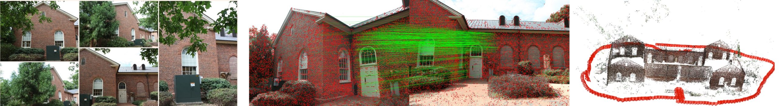
Data collection / Matching features for pairs of images / 3D model
Figure 1: Structure from Motion pipeline. In the final 3D model the cameras are in red and the triangulated points are in black. The reconstruction was done with COLMAP [7] using their data set person-hall.
Multiview varieties
In practice the triangulation is done using noisy data. The noise comes from lens distortion in the cameras, different light effects, or different quality images. This implies that the point or line correspondences obtained in the matching process might not be in the image of the joint camera maps, but are close enough. This is why understanding the images of φ_{C} and ϕ_{C} is necessary. Here is where the multiview varieties come into play.
The Point multiview variety, denoted M_{C}, is defined as the Zariski closure of Im(φ_{C}). Similarly, the Line multiview variety s the Zariski closure of Im(ϕ_{C}).
The point and line multiview varieties are, respectively, the smallest algebraic sets containing all the perfect point and line correspondences. They model perfect data. If we understand these varieties, then we can correct the error of a noisy correspondence by triangulating its closest point in the corresponding multiview variety.
The point multiview variety has been thoroughly studied (see for example [3] or [8] for the basic properties). We highlight the fact that a Groebner basis for its vanishing ideal is known [1] and its Euclidean distance degree is known [5]. For this note we just mention the following theorem from [8] that gives a set of polynomials that cut out the point multiview variety.
Theorem 1. Let C = (C_{1}, . . . , C_{m}) be an arrangement of pinhole cameras, and define the 3m × (m + 4) matrix
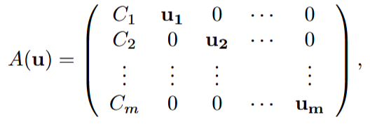
where ![]() for i = 1, . . . , m are the variables associated with the image of each camera. The multiview variety is cut out by the maximal minors of the matrix A(u)
for i = 1, . . . , m are the variables associated with the image of each camera. The multiview variety is cut out by the maximal minors of the matrix A(u)
above.
More recently in [2] the authors start the study of the line multiview variety. They introduce the formal definition that we saw above, provide a set of polynomials that cut out the variety, find its singular locus, and compute its multidegree. The results are given for camera arrangements such that at most four of them are collinear, this means that the they are valid for random camera arrangements or, in the language of Algebraic Geometry, the results are valid generically. We highlight the following theorem from [2]
Theorem 2. Given an arrangement of pinhole cameras C = (C_{1}, . . . , C_{m}), denote by ℓ_{i} the point in the dual of ![]() defining the line υ_{C_{i}}(L) in Gr(1,
defining the line υ_{C_{i}}(L) in Gr(1, ![]() ). The line multiview variety L_{C} is equal to the set
). The line multiview variety L_{C} is equal to the set
![]()
if and only if no four cameras are collinear.
From the geometric point of view, the point multiview variety contains the tuples of points such that their back-projected lines intersect in a point (see Figure 2). Similarly, the line multiview variety contains all the line tuples whose back-projected planes intersect either in a plane or a line (see Figure 3).
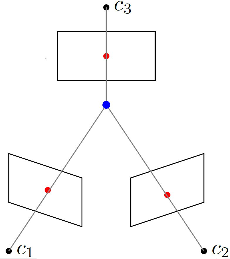
Figure 2: In red a point correspondence for 3 cameras. The back projected
lines of each point are depicted in gray. Since they intersect in the blue point,
the point correspondence is in the point multiview variety M_{C}.
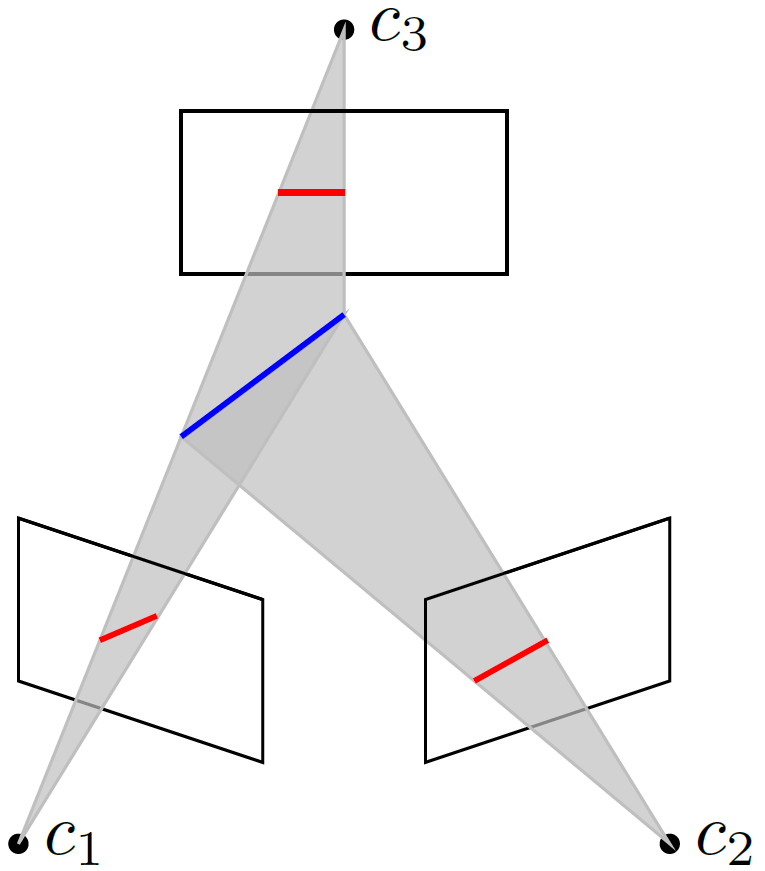
Figure 3: In red a line correspondence for 3 cameras. The back projected
planes of the image lines are depicted in gray. Since they intersect in the blue
world line, the line correspondence is in the line multiview variety L_{C}.
Error correction for real data
In practice, the equations obtained from Theorem 1 and Theorem 2 can be used to develop solvers for triangulation in SfM pipeline. Indeed, triangulating a point cloud requires finding solutions of the same parametric system of polynomial equations as many times as data points. Computer vision engineers have developed implementations that allow for a very fast solution of specific systems coming from theoretical results as the ones introduced above (see for example [4, 6, 7]).
As a final remark we highlight that in [2] the authors conduct numerical experiments to estimate the number of critical points of the distance funcion to the line multiview variety. This is a first approach to the Euclidean Distance degree of the Line multiview variety and it measures the complexity of the triangulation problem using algebraic methods. Although the numerical experiments suggest that this degree is polynomial in the number of cameras, this is still an open question.
References
[1] Chris Aholt, Bernd Sturmfels, and Rekha Thomas, A Hilbert scheme in computer vision, Canadian Journal of Mathematics 65 (2013), no. 5, 961–988.
[2] Paul Breiding, Felix Rydell, Elima Shehu, and Angélica Torres, Line Multiview Varieties, SIAM Journal on Applied Algebra and Geometry 7 (2023), no. 2, 470–504.
[3] Richard I. Hartley, Lines and Points in Three Views and the Trifocal Tensor, International Journal of Computer Vision 22 (1997), no. 2, 125–140.
[4] Shaohui Liu, Yifan Yu, Rémi Pautrat, Marc Pollefeys, and Viktor Larsson, 3D Line Mapping Revisited, Computer Vision and Pattern Recognition (CVPR), 2023.
[5] Laurentiu G. Maxim, Jose I. Rodriguez, and Botong Wang, Euclidean Distance Degree of the Multiview Variety, SIAM Journal on Applied Algebra and Geometry 4 (2020), no. 1, 28–48.
[6] Johannes Lutz Schönberger and Jan-Michael Frahm, Structure-from-Motion Revisited, Conference on Computer Vision and Pattern Recognition (CVPR), 2016.
[7] Johannes Lutz Schönberger, Enliang Zheng, Marc Pollefeys, and Jan-Michael Frahm, Pixelwise View Selection for Unstructured Multi-View Stereo, European Conference on Computer Vision (ECCV), 2016.
[8] Matthew Trager, Martial Hebert, and Jean Ponce, The joint image handbook, Proceedings of the IEEE international conference on computer vision, 2015, pp. 909–917.