(UB), (DMAT, IMTech, CRM), and (CSIC, ICMAT). Received September 26, 2023
1. Introduction
Fundamental to the understanding of physical phenomena and dynamical systems in general is the study of the computational complexity that may arise in a given class of systems. This complexity can include undecidable phenomena and computational intractability, which is relevant not only from a purely theoretical point of view but also in terms of applications to developing algorithms to determine the long-term behavior of a given physical system.
Several dynamical systems have been shown to exhibit undecidable trajectories: there exist explicitly computable initial conditions and open sets of phase space for which determining if the trajectory will intersect that open set can be undecidable from an algorithmic point of view. These include ray tracing problems in 3D optical systems [6], neural networks [7], and more recently ideal fluid dynamics [2, 3], a problem asked in the 90s by Moore [5]. In [3], it was shown that in compact 3D domains, one can find examples of stationary ideal fluids that possess undecidable trajectories. The caveat of the proof is that the Riemannian ambient metric is not canonical in any sense, for instance, the proof does not work to construct such examples in the standard flat three-torus, the standard round sphere, or the standard Euclidean space.
In this note we give a short introduction to the ideas developed in [2], where we construct stationary ideal fluids in the standard Euclidean space ℝ^{3}, i.e., equipped with the flat metric, that possess undecidable trajectories. The price to pay to obtain solutions in a space with a fixed Riemannian metric like the Euclidean one is working on a non-compact space and obtaining solutions that do not have finite energy.
2. Undecidability and Turing machines
The most used technique to prove that a class of dynamical systems might exhibit undecidable trajectories is by constructing an example of that system that is “Turing complete». This means roughly that the system encodes the evolution of any Turing machine, which is a symbolic system encoding a certain algorithm. Let us recall what a Turing machine is.
Turing machines
A Turing machine is defined as T = (Q, q_{0}, q_{halt}, Σ, δ), where Q is a finite set (called “states»), including an initial state q_{0} and a halting state q_{halt}, another finite set Σ called the alphabet of symbols and that contains a blank symbol that we denote by a zero, and a transition function
![]()
that will encode the dynamics (or “algorithm»). A configuration of the machine at a certain step of the algorithm is given by a pair in Q × A, where A denotes the (countable) set of infinite sequences in Σ^{ℤ} that have all but finitely many symbols equal to 0. An “input» of the algorithm, or starting configuration of the machine, is given by a pair of the form (q_{0}, t), where q_{0} is the initial state and t = (t_{i})_{i∈Σ^{ℤ} is an arbitrary sequence in A, which is commonly referred to as the tape of the machine.
The algorithm works as follows. Let (q, t) ∈ Q × A be the configuration at a given step of the algorithm.
- If the current state is q_{halt} then halt the algorithm and return t as output.
- Otherwise, compute δ(q, t_{0}) = (q′, t′_{0}, ε), where t0 denotes the symbol in position zero of t. Let t′ be the tape obtained by replacing t0 with t′_{0} in t, and shifting by ε (by convention +1 is a left shift and −1 is a right shift). The new configuration is (q′, t′), and we can go back to step 1.
We emphasize that there is no loss of generality in the restriction to those sequences A ⊂ Σ^{ℤ} that have “compact support», meaning that all but finitely many symbols are the blank symbol 0. The set P := Q × A is the set of configurations, and the algorithm determines a global transition function
![]()
that sends a configuration to the configuration obtained after applying one step of the algorithm.
Let us finish this section with two more facts about Turing machines. When reproducing an algorithm, one would like to know whether a given Turing machine with a given initial configuration will eventually reach a configuration whose state is the halting state, or if the algorithm will keep running forever. This is known as the halting problem and is known to be (computationally) undecidable as shown by Alan Turing in 1936. This means that there is no algorithm that, given any Turing machine T and any of its initial configurations c, will answer in finite time whether T halts with c or not. A particular consequence of computational undecidability in this context is that for some pairs (T, c), the statement “T halts with c» can be true/false but unprovable, i.e., undecidable in the sense of Gödel.
The second fact that we will need is that there exist “universal Turing machines». Those are Turing machines that can simulate in some sense any other Turing machine, and thus that are capable of reproducing any possible algorithm. One can think of those as a “compiler» in modern computer science. More formally there are different definitions of universal Turing machine, we will use one that is easier to state and that is sufficient for our purposes.
Definition 1. A Turing machine T_{U} is universal if the following property holds. Given any other Turing machine T and an initial configuration c of T there exists an initial configuration c_{U}(T, c) of T_{U} , that depends on T and its initial configuration, such that T halts with c if and only if T_{U} halts with c_{U}.
In particular, determining whether a universal Turing machine with a given initial condition will ever halt is a (computationally) undecidable problem, and there exist initial configurations of T_{U} for which it is (logically) undecidable to determine if T_{U} will halt with that initial configuration.
Turing complete systems
Having understood the relation between Turing machines and undecidability, we relate them to dynamical systems in the following way. Let X be a dynamical system on a topological phase space M, where X can be either discrete or continuous on a finite or infinite-dimensional phase space. For concreteness, we can keep in mind the example of an autonomous flow on a smooth manifold.
Definition 2. A dynamical system X on M is Turing complete if there exists a universal Turing machine T_{U} such that for each initial configuration c of T_{U} , there exists a (computable) point p_{c} ∈ M and a (computable) open set U_{c} ⊂ M such that T_{U} halts with input c if and only if the positive trajectory of X through p intersects U_{c}.
In this case, the halting of a given configuration can be deduced from the evolution of an orbit of X. It is essential to require that p and U_{c} are in some sense explicit, namely computable, since otherwise, one could run into trivial systems being Turing complete. If we are working on a manifold, a point p is computable (in terms of c) if in some chart the coordinates of p can be exactly computed in finite time (in terms of c), for instance having explicit rational coordinates. Computability of an open set U_{c} can be loosely defined as saying that one can explicitly approximate U_{c} with any given precision. This notion is formalized in a subject called computable analysis. A Turing complete system has undecidable trajectories, meaning that there exist an explicit point p and open set U for which determining if the trajectory of p reaches U is an undecidable statement. This is different from being chaotic, where the sensitivity to initial conditions yields a practical unpredictability of trajectories since we are saying that even if we know exactly the initial point p, the long-term behavior can be completely unpredictable.
In practice, most Turing complete systems are constructed in the following way. We first encode, in a computable way, each configuration (q, t) of a universal Turing machine T_{U} as a point or an open set U_{(q,t)} of the phase space M . For our purposes, assume we encode the initial configuration ![]() as points p_{
as points p_{![]() } , and every other configuration as an open set. We then require that for each initial configuration
} , and every other configuration as an open set. We then require that for each initial configuration ![]() , the trajectory of X through p_{
, the trajectory of X through p_{![]() } sequentially intersects the sets corresponding to the configurations obtained by iterating the Turing machine starting with
} sequentially intersects the sets corresponding to the configurations obtained by iterating the Turing machine starting with ![]() . Namely, the trajectory through
. Namely, the trajectory through ![]() will first intersect the set that encodes ∆
will first intersect the set that encodes ∆![]() , then the set that encodes ∆^{2}
, then the set that encodes ∆^{2}![]() and so on, without intersecting any other coding set in between. With this property, we can consider the open set U obtained as the union of all the open sets U_{(q_{halt}, t)} for each t ∈ A, and the trajectory through p_{
and so on, without intersecting any other coding set in between. With this property, we can consider the open set U obtained as the union of all the open sets U_{(q_{halt}, t)} for each t ∈ A, and the trajectory through p_{![]() } will intersect U if and only if the machine T_{U} halts with initial configuration
} will intersect U if and only if the machine T_{U} halts with initial configuration ![]() .
.
3. Constructing stationary ideal fluids that are Turing complete
Having defined Turing complete systems, let us now describe the equations for which we would like to construct a solution that is Turing complete.
The Euler equations and sketch of the main theorem
The motion of an incompressible fluid flow without viscosity is modeled by the Euler equations. In ℝ^{3}, the equations can be written as
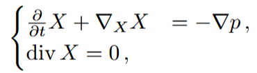
where p stands for the hydrodynamic pressure and X is the velocity field of the fluid (a non-autonomous vector field). Here ∇_{X} X denotes the covariant derivative of X along X. If X is a stationary solution, i.e., time independent, then the first equation is equivalent to ![]() and curl denotes the standard curl operator induced by the Euclidean metric. A vector field that satisfies curl(X) = λX for some constant λ ≠ 0 is called a Beltrami field. It is a particular case of a stationary Euler flow with constant Bernoulli function. The main theorem we proved in [2, Theorem 1] is:
and curl denotes the standard curl operator induced by the Euclidean metric. A vector field that satisfies curl(X) = λX for some constant λ ≠ 0 is called a Beltrami field. It is a particular case of a stationary Euler flow with constant Bernoulli function. The main theorem we proved in [2, Theorem 1] is:
Theorem. There exists a Turing complete Beltrami field u in Euclidean space ℝ{3}.
The strategy of the proof can be sketched as follows.
- We show that there exists a Turing complete vector field X in the plane ℝ^{2} that is of the form X = ∇f where f is a smooth function.
- Furthermore, we require that if we perturb X by an error function ε : ℝ^{2} → ℝ that decays rapidly enough at infinity, then we obtain a vector field that is Turing complete as well.
- We show that a vector field in ℝ^{2} of the form X = ∇g, where g is an entire function, can be extended to a Beltrami field v in ℝ^{3} such that v|z=0 = X. That is v leaves the plane {z = 0} invariant and coincides with X there.
- We approximate f by an entire function F with an error that decays rapidly enough. Hence
 is Turing complete and extends as a Beltrami field u on ℝ^{3}. It asily follows that u is Turing complete as well.
In this note, we will sketch the arguments of steps (1) and (2). The third step is done via a global Cauchy-Kovalevskaya theorem adapted to the curl operator. The fourth step is a general result about approximation of smooth functions by entire functions with errors with arbitrary decay [4].
Weakly robust Turing complete gradient flow in the plane
The goal of this section is to construct a Turing complete gradient flow on ℝ^{2} and sketch how to make sure that its Turing completeness is robust under perturbations that decay fast enough at infinity. Following the recipe explainedin Section 2, we will first show how to encode the configurations and initial configurations of a given universal Turing machine TU into ℝ^{2}. Without loss of generality, we assume that T_{U} = (Q, Σ, q_{0}, q_{halt}, δ) with Q = {1, …, m} for some m ∈ ℕ and Σ = {0, 1}.
he encoding. We first construct an injective map from P = Q × A to I = [0, 1], where we recall that A is the set of sequences in Σ^{ℤ} with finitely many non-zero symbols.
Given (q, t) ∈ P, write the tape as
· · · 000t_{−a} · · · t_{b}00 · · · ,
where t_{−a} is the first negative position such that t_{−a} = 1 and t_{b} is the last positive position such that t_{b} = 1. If every symbol in a negative (or positive) position is zero, we choose a = 0 (or b = 0 respectively). Set the non-negative integers given by concatenating the digits s := t_{−a} · · · t_{−1}, r := t_{b} · · · t_{0}, and introduce the map
![]()
which is injective and its image accumulates at 0. There exist pairwise disjoint intervals I(q,t) centered at φ(q, t), for instance of size 1/4 · φ(q, t)^{2}. To introduce an encoding into ℝ^{2} we proceed as follows. Fix ϵ > 0 small, we encode (q, t) as
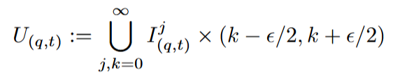
where ![]() . In other words, we are looking at any interval of the form I^{j,k} := [2j, 2j + 1] × {k} ⊂ ℝ^{2}, with j, k ∈ ℕ, and considering an ε-thickening of I_{(q,t)} understood as a subset of I^{j,k} ∼= [0, 1]. Figure 1 gives a visualization of part of one of the open sets U_{(q,t)} in a region of the plane.
. In other words, we are looking at any interval of the form I^{j,k} := [2j, 2j + 1] × {k} ⊂ ℝ^{2}, with j, k ∈ ℕ, and considering an ε-thickening of I_{(q,t)} understood as a subset of I^{j,k} ∼= [0, 1]. Figure 1 gives a visualization of part of one of the open sets U_{(q,t)} in a region of the plane.
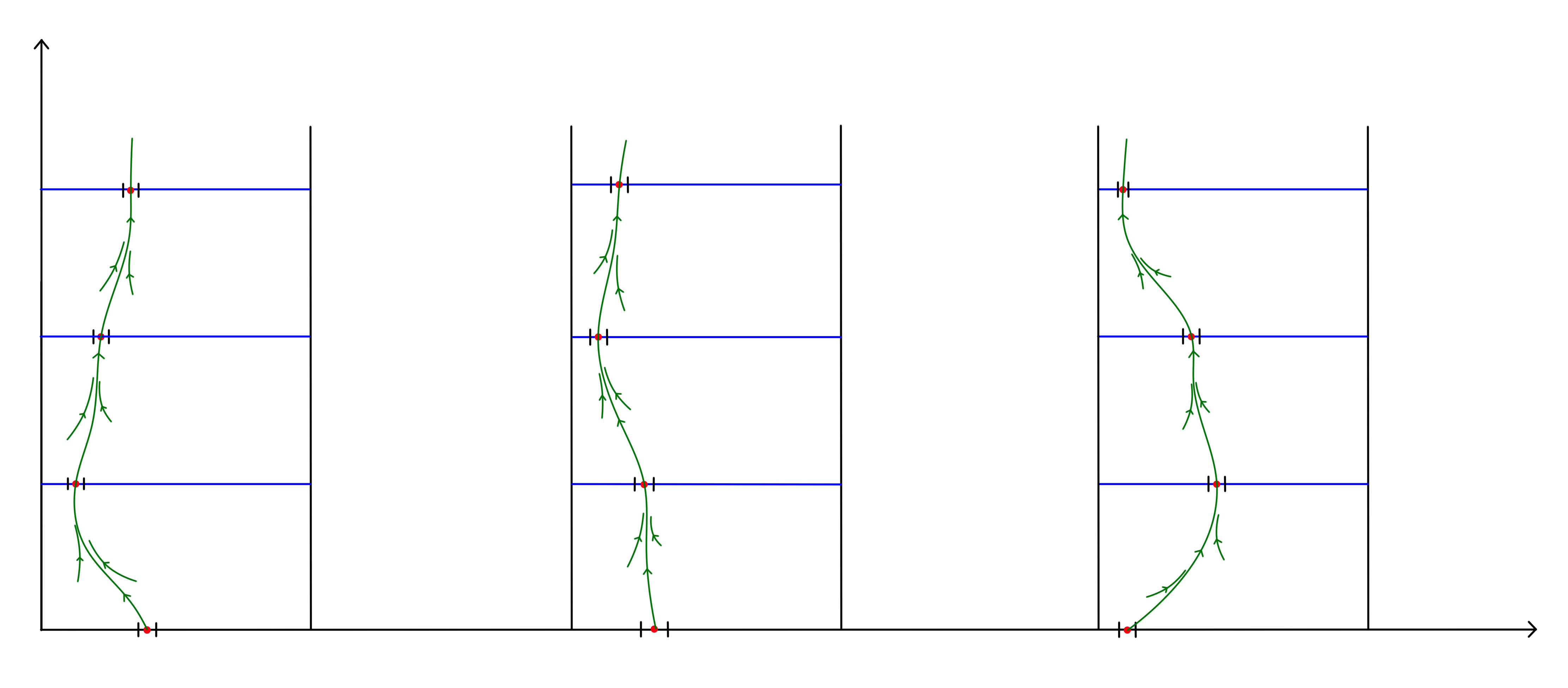
Figure 1. The open set U(q,t) is the ε-thickening of the intervals ![]()
The countable set of initial configurations P_{0} = {(q_{0}, t) | t ∈ A} admits a (computable) ordering which we will not specify, so that we can write it as P_{0} = {c_{i} = (q_{0}, t^{i}) | i ∈ ℕ}. Given c_{i}, the initial condition associated to the vector field that we will construct will be p_{c_{i}} = (φ(c_{i}) + i, 0) ∈ ℝ^{2}. This corresponds to the point φ(q_{0}, t^{i}) of the copy I^{i,0} of the several intervals we considered.
Integral curves capturing the steps of the algorithm. Iterating the global transition function from an initial configuration c_{i} = (q_{0}, t^{i}) gives a countable sequence of configurations ![]() = ∆^{k}(c_{i}) for each k an integer greater than 1. On each band [2i, 2i + 1] × [0, ∞), we construct a smooth curve γ_{i} such that γ_{i} ∩ {[2i, 2i + 1] × {k}} is the point
= ∆^{k}(c_{i}) for each k an integer greater than 1. On each band [2i, 2i + 1] × [0, ∞), we construct a smooth curve γ_{i} such that γ_{i} ∩ {[2i, 2i + 1] × {k}} is the point ![]() , which lies in
, which lies in ![]() , see Figure 2.
, see Figure 2.
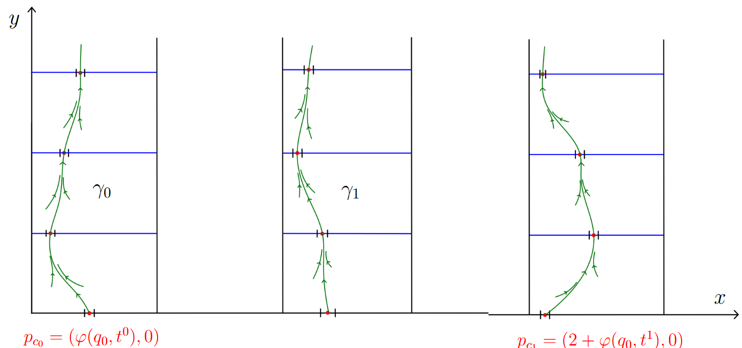
Figure 2. Integral curves following the computations of the Turing machine
We conclude by constructing a gradient field X = ∇f such that each γ_{i} is an integral curve of X. Observe now that given an initial condition c_{i}, the integral curve through p_{c_{i}} will intersect sequentially the open sets ![]() , thus keeping track of the computations of the machine with initial configuration ci. One easily shows that X is Turing complete, where to each c_{i} we assign the initial condition p_{c_{i}} , and the open set U for which the trajectory through c_{i} intersects U if and only if the machine halts with initial configuration c_{i} is simply
, thus keeping track of the computations of the machine with initial configuration ci. One easily shows that X is Turing complete, where to each c_{i} we assign the initial condition p_{c_{i}} , and the open set U for which the trajectory through c_{i} intersects U if and only if the machine halts with initial configuration c_{i} is simply ![]() , that is, every open set encoding a halting
, that is, every open set encoding a halting
configuration.
Weak robustness and conclusion. Recall that in order to apply the Cauchy-Kovalevskaya theorem, we need X to be the gradient of an entire function. To achieve this, we construct X in a way that the flow normally contracts towards each curve γ_{i} at a strong enough rate. This can be used to show that if we perturb X by an error function ε(x, y) with fast decay at infinity, we obtain a vector field that is again Turing complete. This is because even if the curve γ_{i} will no longer be an integral curve, the integral curve through any of the points p_{c_{i}} of the perturbed vector field will still intersect sequentially the open sets ![]() , hence capturing the computations of the Turing machine. The fast decay of the error is necessary since the open sets
, hence capturing the computations of the Turing machine. The fast decay of the error is necessary since the open sets ![]() have no uniform lower bound on their size. This is because the intervals I_{(q,t)} accumulate at zero, and hence their size tends to zero. One can estimate the decay rate of the size of the open sets that need to be intersected by the curves in terms of the distance to the origin, and hence robustness can be achieved under fast decay errors. The construction concludes by approximating f by an entire function
have no uniform lower bound on their size. This is because the intervals I_{(q,t)} accumulate at zero, and hence their size tends to zero. One can estimate the decay rate of the size of the open sets that need to be intersected by the curves in terms of the distance to the origin, and hence robustness can be achieved under fast decay errors. The construction concludes by approximating f by an entire function ![]() (using [4]), and applying the Cauchy-Kovalevskaya theorem for the curl to the Cauchy datum ∇
(using [4]), and applying the Cauchy-Kovalevskaya theorem for the curl to the Cauchy datum ∇![]() on the plane {z = 0}.
on the plane {z = 0}.
References
[1] V. I. Arnold, B. Khesin. Topological Methods in Hydrodynamics. Springer, New York, 1999.
[2] R. Cardona, D. Peralta-Salas, E. Miranda. Computability and Beltrami fields in Euclidean space. J. Math. Pures Appl. 169 (2023) 50–81.
[3] R. Cardona, E. Miranda, D. Peralta-Salas, F. Presas. Constructing Turing complete Euler flows in dimension 3. Proc. Natl. Acad. Sci. 2021, 118 (19) e2026818118; DOI: 10.1073/pnas.2026818118.
[4] E.M. Frih, P.M. Gauthier. Approximation of a function and its derivatives by entire functions of several variables. Canad. Math. Bull. 31 (1988) 495–499.
[5] C. Moore. Undecidability and Unpredictability in Dynamical Systems. Phys. Rev. Lett. 64 (1990) 2354–2357.
[6] J.H. Reif, J.D. Tygar, A. Yoshida. Computability and complexity of ray tracing. Discrete Comput. Geom. 11 (1994) 265–288.
[7] H.T. Siegelmann, E.D. Sontag. On the computational power of neural nets. J. Comput. Syst. Sci. 50 (1995) 132–150.